EN

by Tim Varelmann
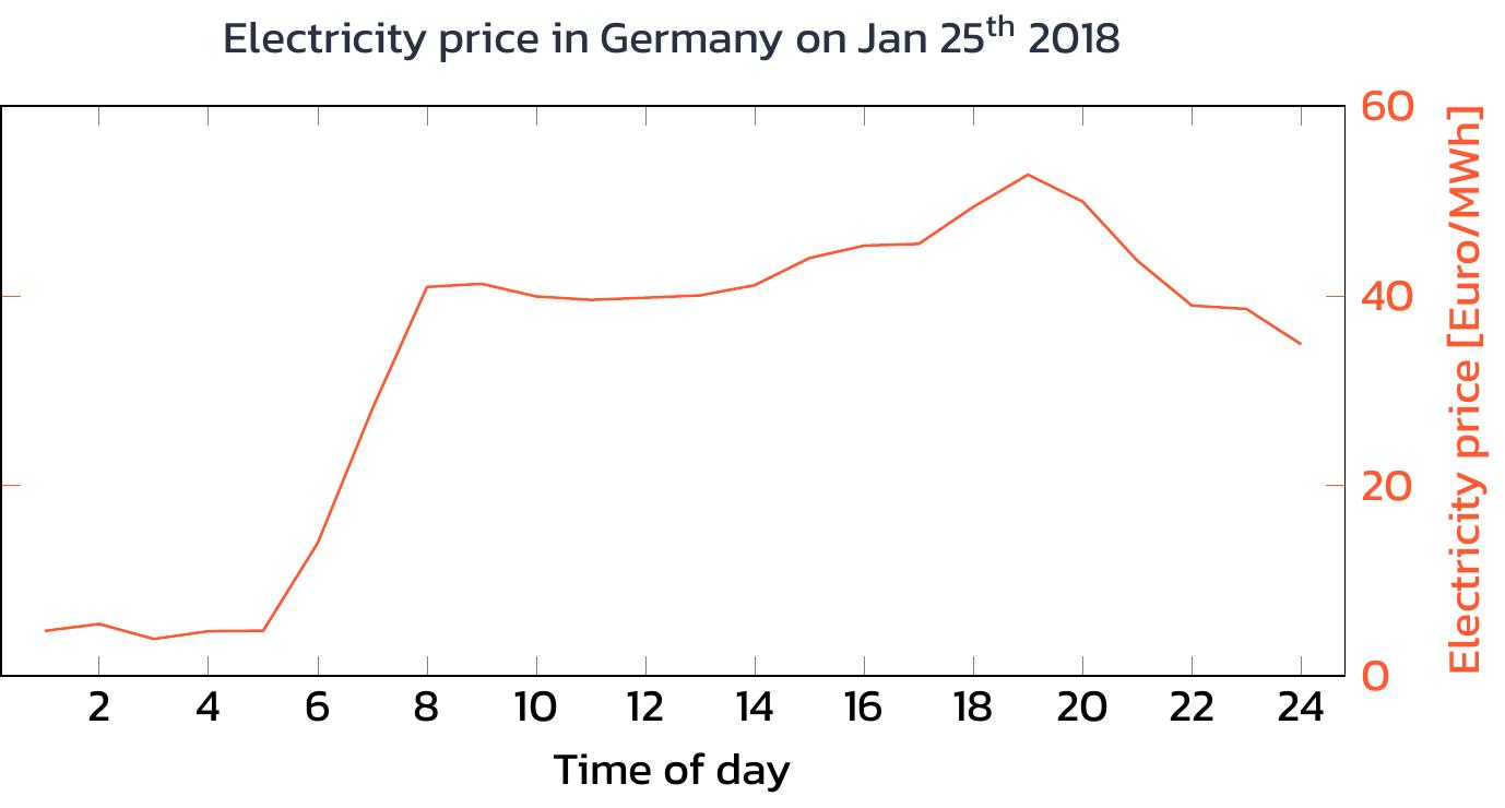
The first two parts of this series have described a simplified model of an aluminum production plant. We now want to use this model to optimally adjust the electricity consumption to the real electricity prices of January 25, 2018. As briefly mentioned in the first part of this series, large electricity consumers have access to the day-ahead market. Therefore, their electricity consumption can be planned one day in advance as the electricity prices for any given day are fixed at mid-day of the previous day already. In practice, very accurate predictions of electricity prices are available for more than one day, so real-world production scheduling often considers a larger planning horizon. Nevertheless, here, we focus on a single day.
Many common optimization algorithms are already implemented in software packages that are either available open-source or sold commercially. Before choosing a suitable algorithm to solve a problem with a given model, it is worthwhile to examine more closely what properties the given model formulation has. We will see that small changes to the given model can change important model properties in such a way that the problem becomes easier to solve.
The simplest class of optimization problems is LPs – Linear Programs. LPs can be solved with very powerful algorithms, which matured over the course of several decades. The solution of auxiliary LPs is also a part of many algorithms to solve the next class of optimization problems: MILPs – Mixed-Integer Linear Programs. In such problems, some variables have a special restriction that their values must be integers. Another way to increase the difficulty of linear programs is to introduce nonlinearities, i.e., some terms in the model use the decision variables in a nonlinear way. Examples for nonlinear uses of a variable x are x2, sin(x) and log(x). It is generally not easy to say whether an NLP is harder to solve than an MILP. Solvers for NLP and MILP can solve many practical application problems with acceptable computational effort and with satisfactory accuracy. Clearly, a problem class that is even harder to solve is a problem comprising both nonlinearities and integer variables. Such problems are called MINLPs – or Mixed-Integer Nonlinear Problems. Current solvers can solve some practically relevant problems already, but algorithms for solving general MINLPs are not even remotely as mature as the algorithms to solve problem instances from the previous classes.
The model presented in the previous part uses the decision variables E[t], T[t] and mAlu[t] in linear terms – except once, when the relation between electrical energy consumption and produced aluminum is described:
mAlu[t] = a3*E[t]3 + a2*E[t]2 + a1*E[t]
Here, E[t] is used in the third and second power, making the model formulation an NLP, since we do have nonlinear terms, but no integer variables. However, we do not have to stick to this formulation. Instead, the function can be approximated as piecewise linear function:
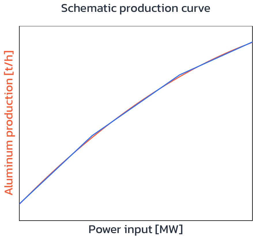
In this picture, we can see that the blue piecewise linear description is an approximation of the orange original nonlinear function. To make the approximation arbitrarily accurate, we can use more than just three linearization intervals. Schäfer et al. have used 15 linearization intervals in [1] to ensure a highly accurate approximation of the originally nonlinear formulation. The reformulation in [1] transformed the problem from an NLP to an MILP which Schäfer et al. found easier to solve. Furthermore, this reformulation allowed me to do another reformulation later on: in [2], I have published an additional trick to reformulate the MILP as LP, which means I was able to reformulate the problem without having to use integer variables. As a consequence, the solution of the LP requires less than a quarter of the runtime required to solve the MILP, which was already faster than the NLP formulation.
This application is a great example for the impact of carefully examining the structure of a model. We could have just put the NLP formulation into an NLP solver and would have probably gotten an optimal production schedule after some computing time. The search for approximations introducing tolerable errors and other tricks, however, enabled the reformulation of the original NLP as an instance of the simplest problem class under the sky: an LP. This allows to solve the production scheduling problem very efficiently, using mature linear programming solvers. Furthermore, the LP formulation has some nice theoretical properties, which allow the production scheduling problem to be integrated into an even bigger decision. For this rather scientific topic, the interested reader is referred to [2].
Finally, let us have a look at how an optimal production schedule looks like for the electricity price profile of January 25 2018:
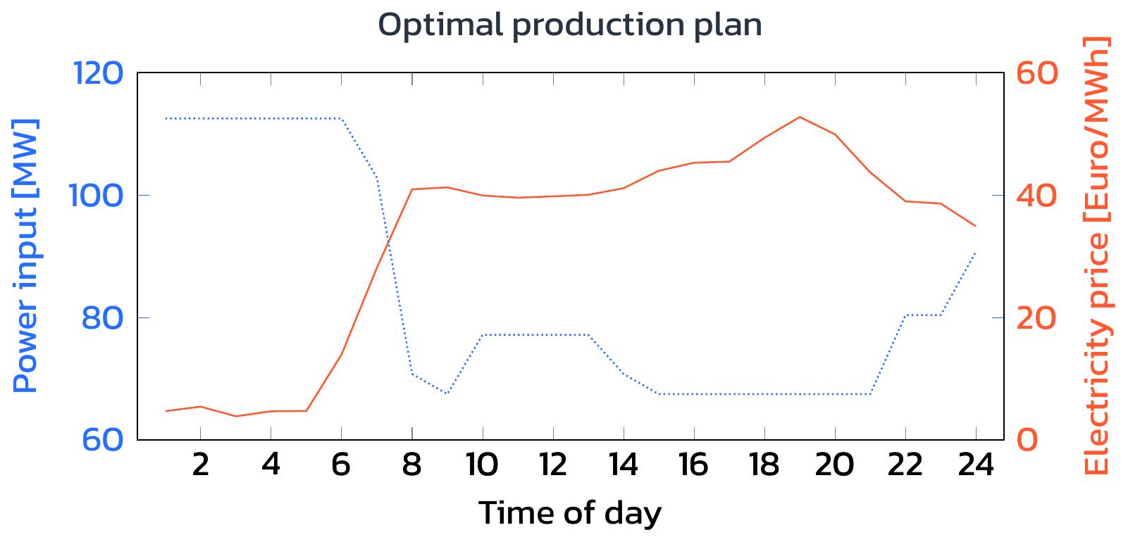
Indeed, we can see that the aluminum plant now produces at maximum capacity most of the night-time where electricity is cheap. Then, when daytime comes, the aluminum plant is able to reduce its energy consumption during peak times, taking stress away from the electricity grid instead of requiring even more fossil power plants to be added to the mix of electricity generators. The average price on 25th January 2018 was a little below 33 Euro/MWh. A constant production strategy with E0 of 90MWh leads to electricity cost of over 71 000 Euro on this day. In contrast, our optimal production plan reduced the electricity cost by around 11 500 Euro to a number slightly below 60 000 Euro. This means a cost improvement by over 15%, while maintaining safety and achieving the usual production target!
Have you got a challenging model or want to make a difficult model extension? Reducing your energy costs by over 15% sounds appealing to you? Maybe all you need is just the right model reformulation! I am happy to contribute my expertise, so reach out and tell me about your challenge.
References:
[1] Schäfer, P., Westerholt, H.G., Schweidtmann, A.M., Ilieva, S., Mitsos, A., 2019. Model-based bidding strategies on the primary balancing market for energy-intense processes. Comput. Chem. Eng. 120, 4–14.
[2] Varelmann, T., Erwes, N., Schäfer, P., Mitsos, A., 2021, Simultaneously optimizing bidding strategy in pay-as-bid-markets and production scheduling. Comput. Chem. Eng. 157, 107610.
Thanks to Simon Thiele for proofreading this article and providing valuable feedback.