by Tim Varelmann

‍

In Part 1 of this series, I described what happens in aluminum production and explained how flexible aluminum production can contribute to the energy transition if the production plan is optimized. Every optimization problem is a description of a complicated decision task. Here, the decision is: How should the aluminum plant produce to have minimal electricity costs without compromising safety and continue to produce the normal mass of aluminum? That sounds actually complicated...

‍

The decision variables

To address these complications, we divide the problem into smaller parts and describe electricity consumption, electricity costs, safety, and production one at a time; and we start with the most important ingredient of the description  — the decision variables. Our decisions are the amounts of electrical energy that the plant uses at each time of the day. We write time as t and the electrical energy consumption at a time t as E[t]. Because we have different prices each hour, we have 24 different relevant times and, thus, 24 energy consumption decisions:

E[1], E[2], E[3], ..., E[24]

To describe the cost of a production plan, we use the hourly electricity prices, which we write as p[t]. The goal of our decision is to minimize electricity costs:

min p[1]*E[1] + p[2]*E[2] + ... + p[24]*E[24]

‍

Plant safety

In order to ensure the safety of the plant, our production plan must guarantee that the mass of liquid aluminum and bauxite is at a temperature that is within a safe range at all times. If the maximum temperature is exceeded, parts of the plant risk melting; if the temperature falls below the minimum, the bauxite-aluminum mass begins to solidify, which is also harmful to the plant. Using the process temperature T[t], we can describe the conditions for safety as:

T[t] < T_max; for all t = 1, ..., 24

T[t] > T_min; for all t = 1, ..., 24

For T_max and T_min, we use numbers from the safety manual of the electrolysis plant. Now we have formulated conditions for the safety of the plant as mathematical inequalities. In this way, a computer can understand what safety means. Now, in order for us to make a decision that takes safety conditions into account, we must also formulate how our decisions affect the temperature of the bauxite-aluminum mass.

‍

As in Springfield, the laws of thermodynamics apply to aluminum electrolysis, in particular the conservation of energy. So, we set up an energy balance to model that the difference between incoming energy and outgoing energy is stored in the process – in the form of thermal energy, which influences temperature.  

Let us denote the energy consumption that the plant would have if the production strategy were constant and inflexible with E⁰. The energy that turns the low-energy bauxite into the high-energy aluminum is outgoing energy. To simplify some electrolysis-related details, we can assume that the outgoing energy is E⁰ as this is how the plant was originally designed [1]. The incoming energy is determined by our decision variables, the electricity consumption in each hour. Finally, the so-called heat capacity C describes how much energy the bauxite-aluminum mass absorbs to raise its temperature by one degree. So, heat capacity is a coefficient with the dimension energy per temperature that describes properties of the material in the plant.

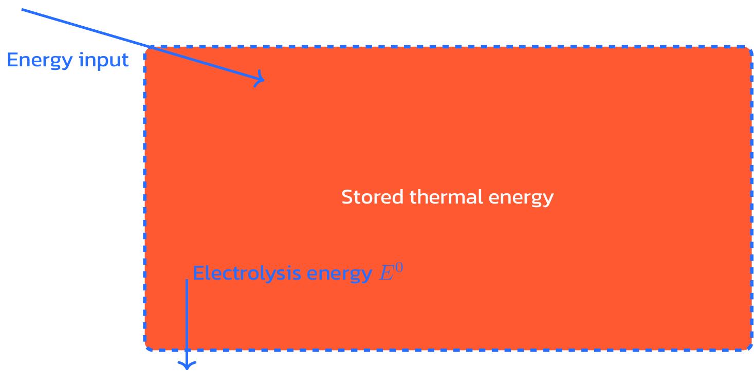
Using all the above, we can write:

T[t+1] - T[t] =  (E[t] - E⁰)/C; for all t = 1, ..., 23

This balance describes that the temperature of the bauxite-aluminum mass rises when we use more electricity than usual, and that the temperature falls again when we use less electricity than usual.

‍

Production

Our model now describes what decisions the production schedule can make, what the goal of the decisions is, and under what conditions the plant produces safely. Finally, we ensure that our flexible production strategy produces enough aluminum to meet the plant's supply contracts. Reusing the superscript-zero, we can denote the hourly aluminum production with a constant and inflexible strategy with m⁰_Alu tons of aluminum per hour. A flexible production strategy should therefore also have an average production of m⁰_Alu, which means the m_Alu[t] have to satisfy:

m_Alu[1] + m_Alu[2] + ... + m_Alu[24] = 24 * m⁰_Alu

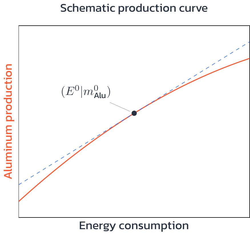
In analogy to T[t], we have introduced new variables m_Alu[t] to describe a condition to the computer. Now, we need further descriptions of how the new variables are affected by our decisions. We already know that production with E⁰ leads to an hourly aluminum production of m⁰_Alu. A first idea might be that if the electricity consumption is increased by – say 20% – there will also be a 20% increase in aluminum production. And in fact, this is roughly true, but not exactly. The reason is that the plant works best when its electricity consumption is E⁰. The plant was designed to run at E⁰ many years ago, when the plan was to produce like that forever. If the plant runs at different levels, there is a slight, but noticeable loss of efficiency. So, if the energy input was increased by 20%, aluminum production would increase by only 19%. And if the energy input is decreased by 20%, aluminum production could decrease by 21%. Additionally, the larger the deviation from E⁰, the larger the efficiency loss. As we might want to produce at maximum and minimum capacity for a substantial fraction of each day, this is an important characteristic of the plant that we have to make the computer aware of with our descriptions. We can describe this effect with the following equations:

m_Alu[t] = a₃*E[t]³ + a₂*E[t]² + a₁*E[t]

Where a₃, a₂, and a₁ are suitable numbers whose values do not help here. Instead, I show a sketch of the described relation:

‍

Implications of the term 'model'

Now, we have collected a bunch of equations and inequalities, which all describe how the optimal production plan we are looking for should look like. This mathematical description is called a ‘model’ of our optimization problem. In contrast to the real-world problem, we have only modeled relevant aspects of reality and made some assumptions that make our lives easier. For example, we assumed a simple description for the electrolysis energy in the energy balance, neglected heat loss to the environment of the plant, and of course the polynomial relation between energy consumption and aluminum production is far from precise in a quantum physical sense...

Strictly speaking, these assumptions are not true, but our description is still close enough to reality that the optimal solution to our slightly unrealistic description of the production schedule is a very good decision in the real world. We can determine the optimal solution at the push of a button, thanks to the simplifying assumptions. This process is described in the next part.

To discuss whether your process can also be modeled mathematically, contact me!

‍

‍

‍

References:

The model described herein is a simplified form of the model developed in [1] and then used, e.g., in [2] and [3].

[1] Schäfer, P., Westerholt, H.G., Schweidtmann, A.M., Ilieva, S., Mitsos, A., 2019. Model-based bidding strategies on the primary balancing market for energy-intense processes. Comput. Chem. Eng. 120, 4–14.

[2] Schäfer, P., Hansmann, N., Ilieva,S., Mitsos, A., 2019. Model-based bidding strategies for simultaneous optimal participation in different balancing markets. In: Computer Aided Chemical Engineering, Vol. 46. Elsevier, pp. 1639–1644.

[3] Varelmann, T., Erwes, N., Schäfer, P., Mitsos, A., 2021, Simultaneously optimizing bidding strategy in pay-as-bid-markets and production scheduling. Comput. Chem. Eng. 157, 107610.

Thanks to Simon Thiele for proofreading this article and providing valuable feedback.